Recommender Systems are designed to suggest relevant items to the users in whatever capacity they are being used. The main goal is to attain a high level of user personalization and therefore end up with better customer service overall. This creates an opportunity for companies to stand out from their competitors in a distinguished manner.
This article is going to walk you through the many paradigms of creating a Recommender System, that will help you glance at their theoretical and practical aspects. To make the explanations as realistic as possible, the Recommender System is created on a dataset that can be found here.
The dataset has very high number of wines that have been rated by several wine enthusiasts. Our job is to use this data to recommend new and suitable wines to any users that might come to us with a small set of preferences.
The article is going to focus on the topics below:
- Data Preprocessing
- Collaborative Filtering
- Content-Based Filtering
- Hybrid Recommender System
Data Preprocessing
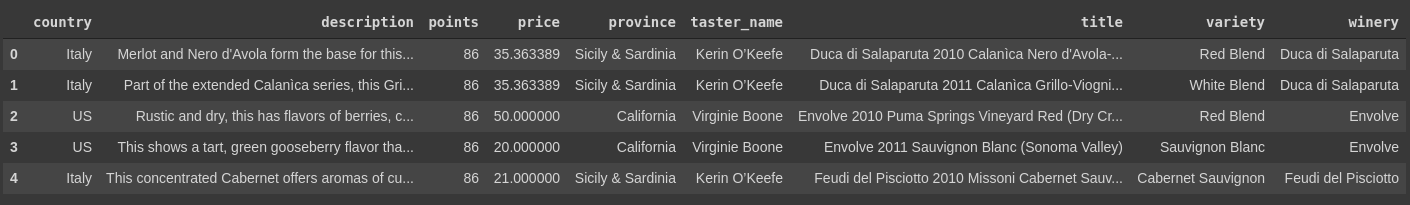
Let us start by looking at the dataset.
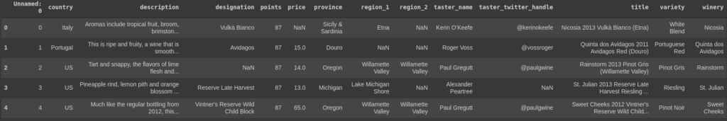
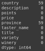
From this table, we can gather important information. There are columns in the data that have incomplete values and we also have some columns which do not seem to contribute important information. We can decide further after we look at the NaN statistics of the data.
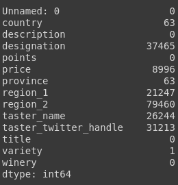
Let us start with fixing the easiest to fix problems and then move forward with the more challenging ones. As can be seen, there is only one missing value in variety, and it can even be filled manually with a google search.
Seems that searching the wine name gave it as Cabernet Sauvignon and it and the variety should be filled as such.
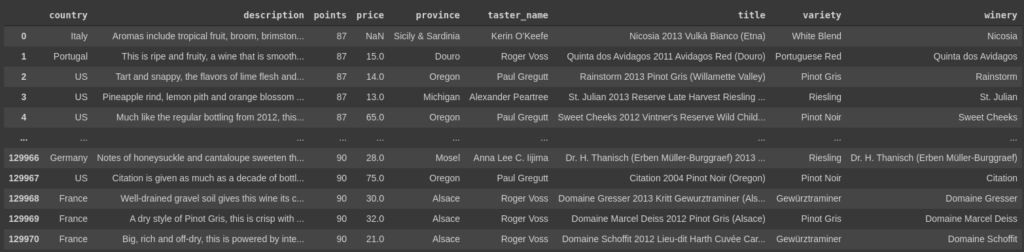
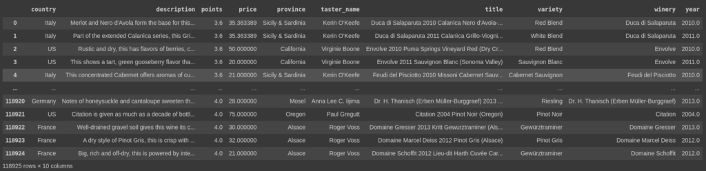
Next, it seems that we need to drop some unnecessary columns. The column ‘Unnamed:0’ is the first one to go as it is just the index of the rows. The columns, ‘designation’, ‘region_1’, ‘region_2’ are also dropped because they have a lot of missing values and would not help a lot. The column ‘taster_twitter_handle’ was also dropped as it did not contribute any useful information. Thus we are left with the following data.
Now our biggest issue seems to be having ratings for some wines but not the person who rated them. That is a must for the model that we want.
The number of unique wines and unique tasters are:
print(len(wineData.title.unique()))
print(len(wineData.taster_name.unique()))
Wines = 118840
Tasters = 19
Since just removing the rows with the unknown tasters would waste precious wine data, some other solution must be used. Before that, we must know if there are any repeated (‘title’, ‘taster_name’) values. This would mean that one taster tasted the same wine and multiple times and we do not need that.
WineData.groupby(['taster_name', 'title']).size().reset_index(name='counts')['counts'].value_counts(dropna=False)
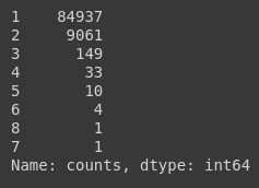
This shows how many (‘title’, ‘taster_name’) pairs have been repeated how many times. For example, 9061 pairs have been repeated twice. Even though it is just one, we have a pair that has been repeated 7 times. Let us just drop all the duplicate rows so we only have unique (‘title’, ‘taster_name’) pairs. Be careful to remove the rows with NaN tasters before dropping and then reattaching them after dropping.
We are back to our NaN tasters problem. One viable solution would be to train a model to assign each wine to the current tasters we have according to their previous choices of ratings. The other solution is to create a new taster and assign all of the wines to that taster.
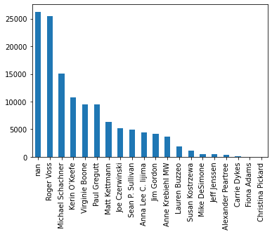
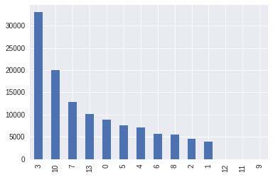
As can be seen from the graph, the taster with the highest number of wines has around 25000 wines. Making another taster would mean that all the NaN wines would go to him/her which are around 26000. Thus making him/her the person who has rated the most wines. Another problem would be that his/her rating would not be consistent as the ratings would be from many different unknown tasters. Thus the most viable solution is to get a model to categorize the wines to different tasters.
The idea is to use SVM with ‘RBF’ kernel to categorize the wines to one of the 19 tasters. The feature space would contain the columns, ‘title’, ‘variety’, ‘winery’, ‘province’, ‘price’, ‘points’. Since there are NaN values in the price, fill them with the mean value of the price. This is not supposed to be a rundown on how to use SVM so let us just skip to the part where we tune the hyper params of our SVM with GridSearchCV.
X = train_test.drop(['taster_name'], axis=1)
y = pd.DataFrame(train_test['taster_name'])
X_train, X_test, y_train, y_test = train_test_split(X, y, test_size=0.3, random_state=0, stratify=y)

params_grid = [{'kernel': ['rbf'], 'gamma': [1e-3, 1e-4],
                     'C': [1, 10, 100, 1000]}]

svm_model = GridSearchCV(SVC(), params_grid, cv = 4)
svm_model.fit(X_train_scaled, y_train)
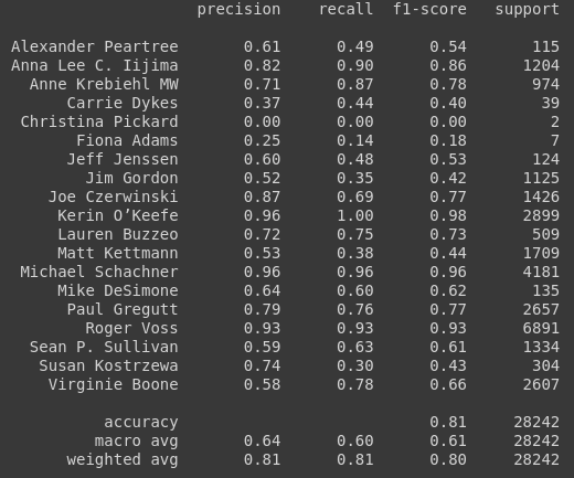
The classification report below on the test set shows that our avg f1 score is around 0.80 which is pretty good considering the features were not that well thought out.
After getting the model to assign the wines to other tasters, and dropping any repeated (wine, taster) pairs we are left with the following tally for the number of wines the tasters have rated.
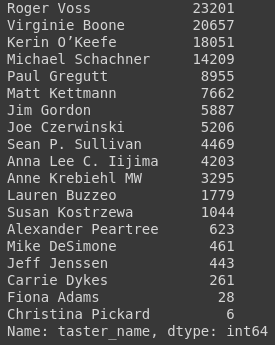
The final value of unique wines we have comes out to 118840. And the number of ratings we have available are 120440. Meaning that there are very little wines that have been rated twice but that is a problem for later. Our NaN counts should look like this:
Since we only have NaN values in the country and province, and we do not need country in collaborative filtering, the data set at this point is as below:
The Ratings that we have are from 80 – 100 with a scale of 0 – 100 and since we want the rating scale to be as general as possible, so the scale was chosen as 0 – 5, and the 80 – 100 values were translated to 3 – 5.
x = (WineData1['points'] - WineData1['points'].mean())/WineData1['points'].std()
x = x - x.min()
x = x / x.max()
x = (x * 2) + 3
WineData1 = WineData1.assign(points=x)
Also, the year was extracted from the title of the wine to make a new column.
years = [re.findall(r'[12][0-9]{3}', tit) for tit in WineData1['title']]
i = 0
for year in years:
  if len(year) > 0:
    WineData1.loc[i, 'year'] = str(np.array(list(map(int, year))).max())
  i += 1
The finalized dataset is as follows:
Collaborative Filtering
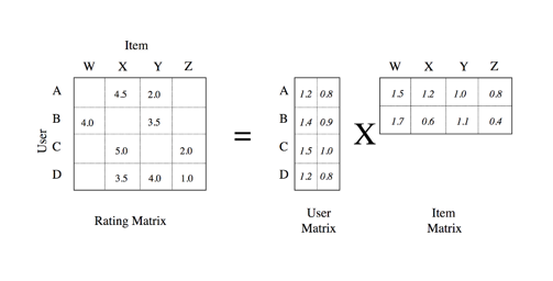
The basic aim of a Collaborative Filtering system is to predict the estimated rating of a user for an item that has not yet been rated by the user. Thus, if there are N number of items, and the user rates C of those items, where (C < N), then the rating of the (N – C) remaining items can be estimated to suggest to the user some items which are highly estimated.
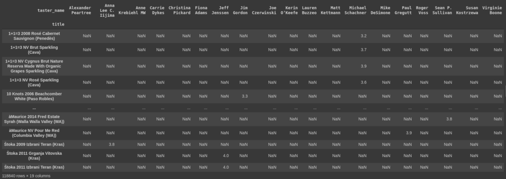
As it can be seen in the user-wine matrix above, the users (columns) have rated some wines but most of the wines have not been rated. If the current matrix can be filled in some way, we would know what these current users would rate these wines and then wines can be recommended to them. To fill this matrix, a technique called matrix factorization is used. This technique requires that we have 2 such matrices which can result in the user-wine matrix when multiplied. These 2 matrices have latent(hidden) features regarding the wines, and the users. If we have N users and M wines, then our user-wine matrix is (M x N). Our 2 matrices should have sizes (M x k) and (N x k) where k is a hyper parameter.
Surprise is a handy library which has several Matrix Factorization based algorithms. Choosing the best algorithm depends on what suits your data the best. Some of these algorithms are, SVD, SVD++ and NMF.
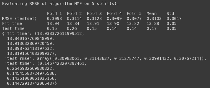
NMF:
algo2 = NMF()
cross_validate(algo=algo2, data=data, measures=['RMSE'], cv=5, verbose=True)
SVD:
algo = SVD()
cross_validate(algo=algo, data=data, measures=['RMSE'], cv=5, verbose=True)
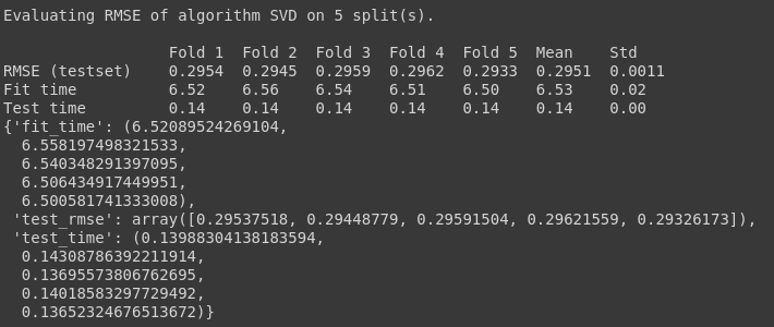
Cross Validating the 2 algorithms, SVD and NMF, we can see that the RMSE(root mean squared error) of SVD is less than that of NMF and it also takes less time to fit the train set. Thus our choice of algorithm is SVD. Choosing the algorithm is not the end of the decisions that have to be made.
We also have to choose the value of k(number of latent factors), learning rates, and regularizations for the model learn. Thus we use GridSearchCV to find the best suitable values for us.
param_grid = {'n_factors' : [35, 50, 75], 'lr_all' : [0.1, 0.01, 0.003], 'reg_all' : [0.06, 0.04, 0.02]}

gs = GridSearchCV(algo_class=SVD, measures=['RMSE'], param_grid=param_grid)
gs.fit(data)
Finally training the final model on the best hyper parameters and then predicting the missing values of the user-wine matrix.
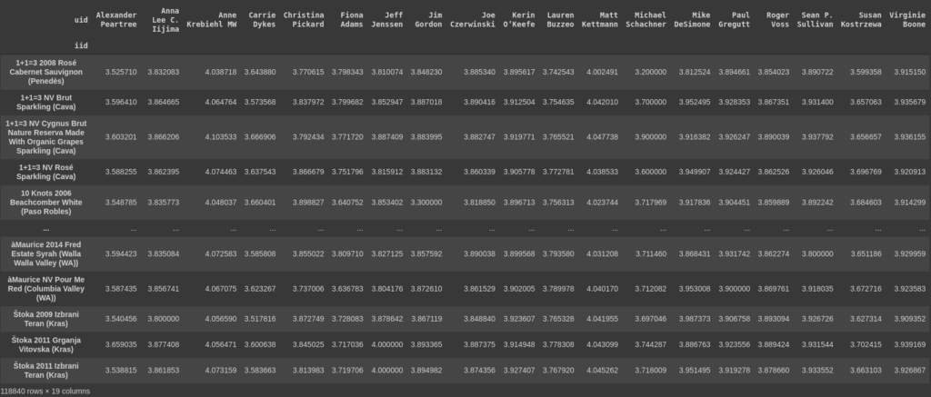
Since our task is not limited to finding out the missing ratings of the registered users, we have to find out a way to find out the ratings of a user which gives a sample of his/her ratings and requests estimated ratings for unrated wines. Performing Matrix Factorization on N users and M wines takes a long time and the user might not want to wait that long. Thus, we find the user who has the most similar ratings, from the filled user-wine matrix, to the new user and then perform matrix factorization on the 2 users to get the missing ratings for the new user. The nearest user in ratings to the new user is found by plotting the ratings in subject of all users in an n dimensional graph where n is the number of wines on which the similar user has to be found.
nearNiegh = NearestNeighbors(n_neighbors=1, algorithm= 'brute', metric= 'cosine').fit(csr_matrix(newPred[:-1, :]))
distance, ind = nearNiegh.kneighbors(csr_matrix([newPred[-1, :]]))
This ensures that the new User gets his/her predicted ratings, according to the behaviour of the user most similar to him/her and skewed according to his/her biases.
To Finalize, when a few rated wines of a user are given the Collaborative filtering model, it gives back the whole wine list with the estimated ratings according to that user.
Content Based Filtering
The basic aim of Content Based Filtering is to find items that are similar to an item in question. This similarity is not based on the ratings of the users but rather the attributes of the items. In our case, wines can be similar to each other by having similar Country, production winery, production year, variety and a somewhat similar description.
The case of country, winery, variety and year is simple as the wines sharing the attributes will be similar in one way or the other. Since all wines have unique descriptions, finding similarity based on description can be challenging.
The descriptions of the wines typically have some similar words regarding their aroma, the fruits used, or the acidity of the wine. Description similarity can be based on these specific words being in the description or not. To turn these descriptions from natural language to numerical form, Tf-idf is used. Tf-idf takes the inverse of the frequency of a specific word and then fills a Tf-idf matrix with these inverses. This matrix is of shape M x D where M is the number of wines and D is the number of words which are selected through Tf-idf.
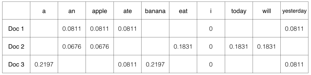
The TfidfVectorizer from sklearn helps create this Tfidf matrix through removing extra useless words and selects the important words for you to have in the matrix.
descrip = wines['description']
idfVector = TfidfVectorizer(max_df=0.8, min_df=1, stop_words='english', lowercase=True, use_idf=True, norm=u'l2', smooth_idf=True)
tfidf = idfVector.fit_transform(descrip)
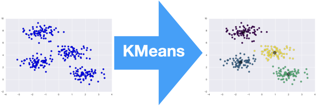
This Tf-idf matrix can be used to plot the wines in an n-dimensional space where n is D in the Tf-idf matrix. The plot can be then used to create k means clusters of wines in the n-dimensional space. The more dense the wines in a cluster, the more similar they are to each other. Also, k nearest wines to a specific wine can be also found.
To determine the number of clusters required, the elbow rule is used. At first, a large number of clusters are created and the number of wines in those clusters are shown in the form of a bar graph.
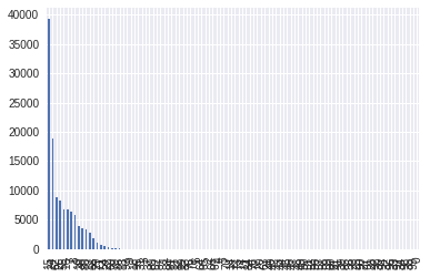
Looking at the graph, we can figure out that after 14 or so clusters, the number of wines in a cluster are negligible, thus, only 14 clusters were made and the model was retrained to have all of the wines in either of these clusters.
This means that instead of having a description in front of every wine, we will have a number from 1 – 14 and since there are above 10000 wines, we can find a great number of similar wines in a cluster.
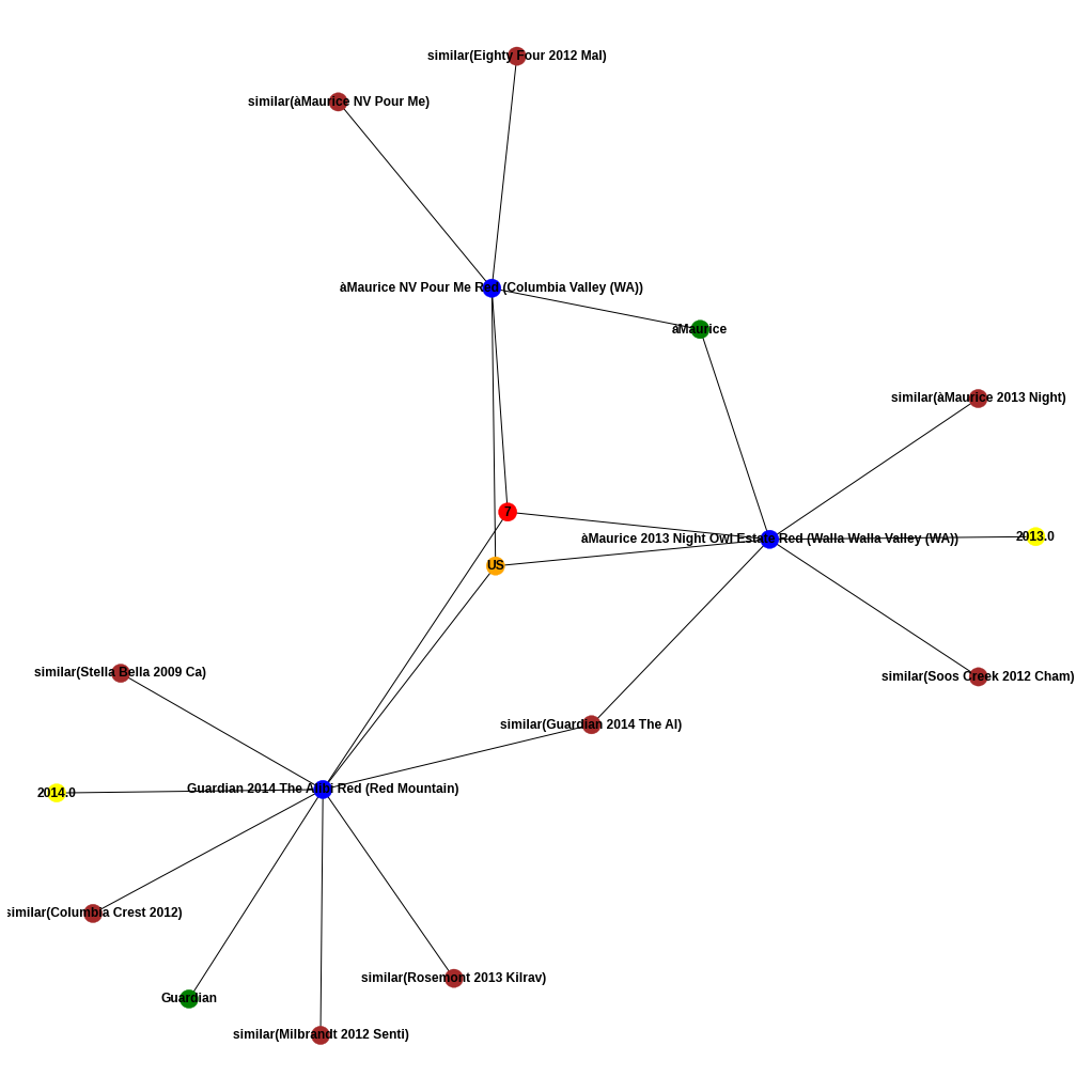
Since natural language restrictions have been removed from the data, similar wines can be found using their attributes, given a certain wine. To accomplish this task, a network is required. A network is such that it has nodes and connections between nodes. What we require is a non directed network with the following as nodes:
- Unique names of wines
- Unique years in which the wines were created
- Unique wineries in which the wines were created
- Unique Countries the wines are from
- Unique variety of the vines
- Unique cluster the wine belongs to
This means that if there is a node of Country(Italy), all the wines which have Italy as an attribute would be connected to Italy. This would create a path from wine a to wine b, thus allowing exploration of different wines from one wine node.
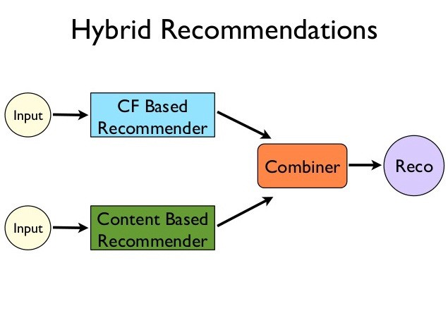
Hybrid Recommender System
The two modules discussed above are used together to create the hybrid recommender system. One of the approaches to using these 2 together is to find the top n similar wines to the highest rated wines in the users original ratings. Using these similar wines, find the top few rated wines using the Collaborative Filter and then recommend them to the user.